stage 08
训练
Training
Inktoys Engrave Everything — 3DGS Tutorial Series · Chapter 08 · Training
Concept and Positioning
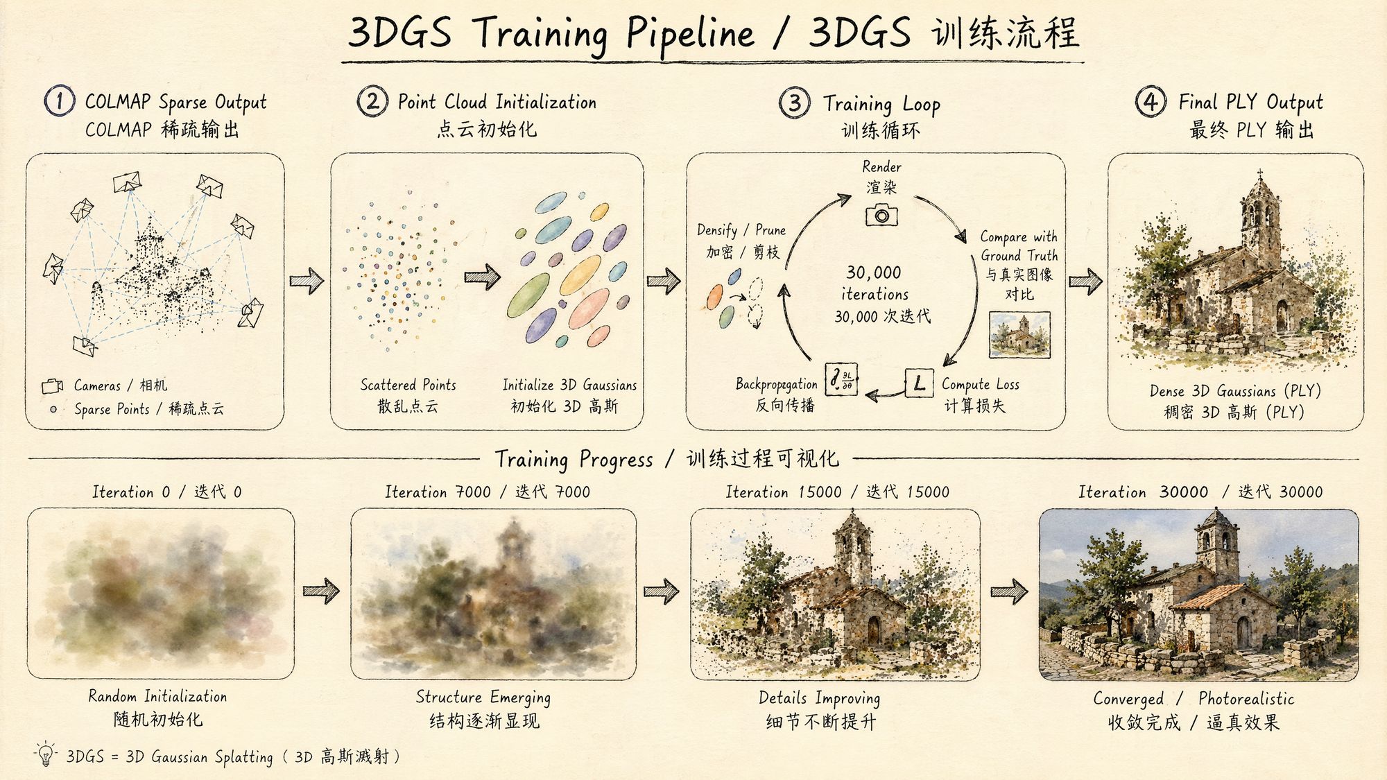
Training is the "magic happens here" step of the 3DGS pipeline. Every previous chapter—capture, frame extraction, color grading, SfM—has been preparing inputs for this moment. The essence of training is this: starting from the sparse point cloud produced by SfM, use differentiable rendering and gradient descent to optimize a few thousand initial 3D Gaussians into millions of Gaussian ellipsoids that precisely describe the scene's appearance.
Each Gaussian carries the following attributes:
• Position (x, y, z): the center point in 3D space
• Covariance matrix (parameterized by scale + rotation quaternion): controls the ellipsoid's shape and orientation
• Opacity: transparency between 0 and 1
• SH coefficients (spherical harmonics): encode view-dependent color information
The core logic of the training loop:
-
From the current Gaussian set, render an image using a differentiable rasterizer
-
Compute the loss between the rendered image and the corresponding ground-truth photo (L1 + SSIM)
-
Backpropagate gradients and update every Gaussian's parameters
-
Periodically run adaptive density control: split/clone Gaussians in high-gradient regions, prune Gaussians with low opacity
-
Repeat for 30,000 iterations
The output after training: a PLY file containing the complete parameters of hundreds of thousands to millions of Gaussians. That file is your 3D scene—it can be rendered in real time from any viewpoint.
Decision Points
Decision 1: Cloud Training vs Desktop Training
This is the most fundamental choice in this chapter. Each path fits a different scenario:
Cloud option: upload images/video, wait for the server to process, download the result. No GPU required.
Desktop option: run training on your local machine. Requires an NVIDIA GPU (minimum 6 GB VRAM).
| Dimension | Cloud | Desktop |
|---|---|---|
| GPU requirement | None | NVIDIA RTX 2060+ |
| Control | Low (black box) | High (fully tunable) |
| Privacy | Data uploaded to a third party | Data never leaves your machine |
| Cost | Subscription or per-job | One-time hardware investment |
| Quality ceiling | Good (~27.5–27.8 dB PSNR) | Highest (~28.1–28.4 dB PSNR) |
| Learning value | Low | High (you understand the training process) |
| Best for | Quick results, no-GPU users | Quality-driven users, parameter tuning, research |
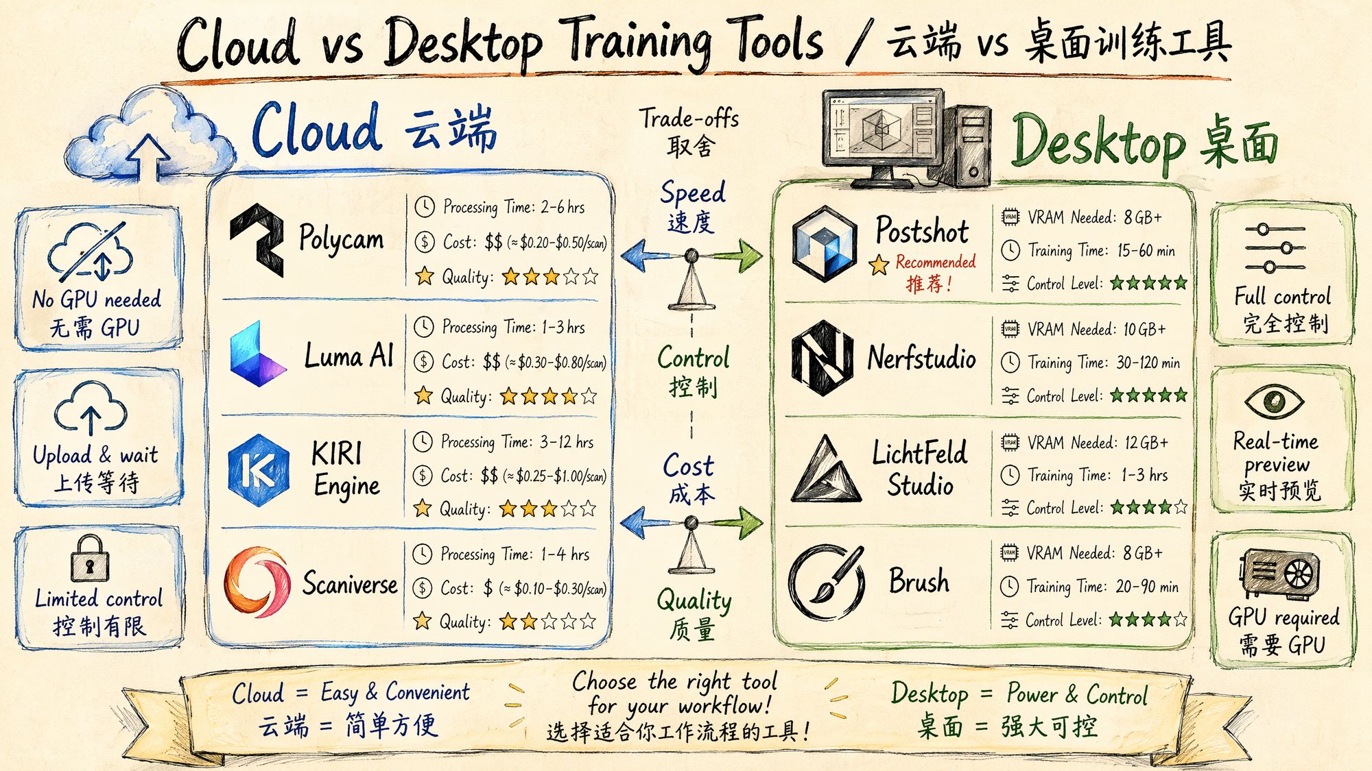
Decision 2: Cloud Options Compared
| Tool | Price | Processing time | Quality | Export formats | Highlights |
|---|---|---|---|---|---|
| Polycam | $8/month Pro | 15–45 min | ★★★★ | PLY, OBJ, FBX, USDZ and 15+ formats | LiDAR support, floor plans, UE5 integration |
| Luma AI | Free basic tier | 3–5 min | ★★★★☆ | PLY | Fastest processing, best visual quality, zero barrier to entry |
| KIRI Engine | $10/month | 30–90 min | ★★★☆ | PLY, OBJ | LiDAR integration, 3 free scans |
| Scaniverse (Niantic) | Free | 5–10 min (on-device) | ★★★☆ | SPZ, PLY | Fully on-device processing, no upload required |
| Teleport | Per-project pricing | Varies | ★★★★ | PLY, SPLAT | Professional grade, supports large scenes |
| Pointcosm | Free beta | 15–30 min | ★★★☆ | PLY | Emerging platform, continuously improving |
Selection guide:
• Want the fastest and easiest → Luma AI (free, results in 3 minutes, excellent quality)
• Need professional export formats → Polycam (15+ formats, LiDAR, floor plans)
• Fully offline / privacy first → Scaniverse (on-device processing, no data upload)
• Tight budget → Luma AI free tier + Scaniverse free tier
Decision 3: Desktop Options Compared
| Tool | Price | Minimum GPU | Training time (83 images) | Quality | Highlights |
|---|---|---|---|---|---|
| PostShot ⭐ recommended | €17/month Indie | RTX 2060 | ~15 min (4090) | ★★★★ | Real-time preview, RealityScan import, UE5 plugin, best GUI |
| Nerfstudio (splatfacto) | Free, open source | RTX 3060 (8 GB) | ~25 min (3060) | ★★★★ | Research framework, multiple methods, active community |
| LichtFeld Studio | Free, open source | RTX 2060 (NVIDIA only) | ~10 min (4090) | ★★★★☆ | Fastest speed, native C++/CUDA, Python plugins, MCP automation |
| Brush | Free, open source | Any GPU (incl. AMD/Intel) | ~20 min | ★★★★ | Cross-platform, hardware-agnostic, WebGPU |
| gsplat | Free, open source | RTX 3060 | ~20 min (3060) | ★★★★☆ | PyTorch library, most modular, 4× memory savings |
| Original 3DGS (INRIA) | Free, open source | RTX 3090 (24 GB recommended) | ~30 min (3060) | ★★★★★ | Reference implementation, highest baseline quality, academic standard |
Inktoys' recommended ranking:
-
PostShot — if you want the "best experience". The real-time training preview lets you watch Gaussians densify and refine progressively, which is invaluable for understanding the training process. Supports importing poses from RealityScan, skipping the COLMAP wait. Excellent GUI design—pause/resume/parameter tweaking are all intuitive.
-
LichtFeld Studio — if you chase "maximum speed + open source". Native C++/CUDA implementation, training speed crushes Python solutions. Supports MCMC strategy and ImprovedGS+ and other cutting-edge algorithms. The Python plugin system allows custom extensions.
-
Nerfstudio — if you are a "researcher/developer". The most complete research framework, supporting splatfacto, instant-ngp, nerfacto and many other methods. End-to-end from data processing to training. The most active community and the first choice for paper reproduction.
-
Brush — if you "do not have an NVIDIA GPU". The only desktop training tool that supports AMD, Intel, and even Apple Metal. Built on WebGPU, truly cross-platform.
Decision 4: Number of Training Iterations
| Iterations | Use case | Quality | Time (RTX 4090) |
|---|---|---|---|
| 7,000 | Quick preview / test | 60–70% of final quality | 2–3 min |
| 15,000 | Medium quality | 85–90% of final quality | 5–6 min |
| 30,000 | Standard full training | 100% baseline | 8–12 min |
| 50,000+ | Extreme quality / difficult scenes | Marginal gains (diminishing returns) | 15–20 min |
Inktoys' suggestion: first run 7,000 iterations to confirm there are no obvious issues (incorrect poses, poor input quality), then run the full 30,000. Going beyond 30,000 is usually not worth the extra time.
Operating Steps
Plan A: PostShot Workflow (Recommended for Beginners)
PostShot currently offers the best GUI experience among 3DGS desktop training tools. Here is the complete workflow:
Step 1: Import Data
Method A: import images/video directly
-
Open PostShot → New Project
-
Drag in an image folder or video file
-
PostShot automatically invokes its built-in COLMAP for SfM
-
Wait for pose estimation to finish (progress bar shown)
Method B: import RealityScan/COLMAP poses (recommended)
-
In RealityScan, complete alignment → Export → COLMAP format
-
PostShot → Import → COLMAP Sparse Model
-
Select the sparse/0/ directory and the images/ directory
-
Poses load directly, skipping the SfM wait
Step 2: Configure Training Parameters
PostShot's defaults are already good for most scenes, but the following parameters are worth attention:
| Parameter | Default | Tuning advice |
|---|---|---|
| Stop Step | 30,000 | Drop to 7,000 for quick previews |
| Max Splat Count | Auto | Limit to 500K for small objects, raise to 5M for large scenes |
| SH Degree | 3 | Keep default (higher SH order = better view-dependent effects) |
| Densification Interval | 100 | Keep default |
| Position Learning Rate | 0.00016 | Keep default |
| Opacity Reset Interval | 3000 | Keep default |
Step 3: Start Training & Monitor in Real Time
-
Click the Train button
-
Watch the live preview window—you will see Gaussians evolve from a sparse point cloud into a complete scene
-
Monitor the training curves:
◦ Loss should keep decreasing
◦ Splat Count should grow quickly at first, then stabilize
◦ PSNR should keep increasing (> 25 dB is acceptable, > 28 dB is excellent)
- If you spot problems, you can Pause at any time:
◦ Floaters appearing → lower the opacity threshold
◦ Insufficient density → raise the densification gradient threshold
◦ Overfitting → reduce iterations
Step 4: Export
After training:
-
File → Export → Gaussian Splat (.ply)
-
Choose the export path
-
Optional: also export the camera trajectory (for later rendering)
PostShot export formats:
• PLY (standard Gaussian Splat, compatible with all viewers)
• SPLAT (compressed format, suitable for the Web)
• Direct Unreal Engine import (via the PostShot UE5 plugin)
Plan B: Nerfstudio splatfacto Workflow (Recommended for Research)
# Prerequisite: ns-process-data already complete (see Chapter 07)
# Train splatfacto (Nerfstudio's 3DGS implementation) ns-train splatfacto \
--data ./processed/ \
--output-dir ./splat_output/ \
--max-num-iterations 30000 \
--pipeline.model.cull-alpha-thresh 0.005 \
--pipeline.model.densify-grad-thresh 0.0002 \
--pipeline.model.sh-degree 3
# During training you can open the Viewer # Visit http://localhost:7007 in a browser to watch live training progress
Key parameters explained:
# Core training parameters --max-num-iterations 30000
# Total iterations --pipeline.model.sh-degree 3
# SH degree (0=flat color, 1=simple lighting, 3=full view-dependent effects)
# Density control parameters --pipeline.model.densify-grad-thresh 0.0002
# Densification gradient threshold (lower = more splits) --pipeline.model.cull-alpha-thresh 0.005
# Pruning opacity threshold --pipeline.model.densify-until-iter 15000
# Densification cutoff iteration --pipeline.model.densify-from-iter 500
# Densification start iteration
# Learning rates --pipeline.model.position-lr-init 0.00016
# Initial position learning rate --pipeline.model.position-lr-final 0.0000016
# Final position learning rate --pipeline.model.feature-lr 0.0025
# Color feature learning rate --pipeline.model.opacity-lr 0.05
# Opacity learning rate --pipeline.model.scaling-lr 0.005
# Scale learning rate --pipeline.model.rotation-lr 0.001
# Rotation learning rate
Export PLY after training:
# Export as standard PLY ns-export gaussian-splat \
--load-config ./splat_output/splatfacto/CONFIG_TIMESTAMP/config.yml \
--output-dir ./export/
Plan C: LichtFeld Studio Workflow (Recommended for Speed)
LichtFeld Studio is a high-performance native C++/CUDA implementation with extremely fast training.
Installation
Download the Windows binary from portal.lichtfeld.io, or build from source on GitHub:
git clone https://github.com/MrNeRF/LichtFeld-Studio.git cd LichtFeld-Studio # Build per the README (requires CUDA 12+, CMake, Visual Studio 2022)Training Workflow
-
Open LichtFeld Studio
-
File → Open Dataset → choose the COLMAP sparse directory
-
Pick a training strategy:
◦ ADC (Adaptive Density Control): the classic 3DGS strategy
◦ MCMC: a newer Markov Chain Monte Carlo strategy that often converges faster
◦ ImprovedGS+: the latest high-performance strategy
-
Click Train → watch the reconstruction in real time
-
When training is done → Export PLY
Unique Advantages of LichtFeld
• Python plugin system: write Python scripts to extend functionality
• MCP automation: external automation via the Model Context Protocol
• Multiple training strategies: switch between ADC / MCMC / ImprovedGS+ for comparison
• Checkpoint resume: resume training from any iteration
Plan D: gsplat Code-Level Training (Recommended for Developers)
gsplat is a low-level CUDA-accelerated library developed by the Nerfstudio team, offering maximum flexibility:
#!/usr/bin/env python3 """ 08_train_gsplat.py Inktoys · 3DGS training with gsplat """
import torch import numpy as np from pathlib import Path from gsplat import rasterization from gsplat.strategy import DefaultStrategy import pycolmap
def load_colmap_data(colmap_path: str, image_dir: str):
"""Load training data from COLMAP output"""
reconstruction = pycolmap.Reconstruction()
reconstruction.read(colmap_path)
# Extract camera intrinsics
camera = list(reconstruction.cameras.values())[0]
K = np.array([
[camera.focal_length_x, 0, camera.principal_point_x],
[0, camera.focal_length_y, camera.principal_point_y],
[0, 0, 1]
])
# Extract image extrinsics and paths
viewmats = []
image_paths = []
for img in reconstruction.images.values():
if not img.registered:
continue
# World-to-camera transform
R = img.rotmat()
t = img.tvec
viewmat = np.eye(4)
viewmat[:3, :3] = R
viewmat[:3, 3] = t
viewmats.append(viewmat)
image_paths.append(Path(image_dir) / img.name)
# Extract initial point cloud
points = []
colors = []
for point in reconstruction.points3D.values():
points.append(point.xyz)
colors.append(point.color / 255.0)
return {
"K": torch.tensor(K, dtype=torch.float32),
"viewmats": torch.tensor(np.array(viewmats), dtype=torch.float32),
"image_paths": image_paths,
"points": torch.tensor(np.array(points), dtype=torch.float32),
"colors": torch.tensor(np.array(colors), dtype=torch.float32),
"width": camera.width,
"height": camera.height,
}
class GaussianModel:
"""3D Gaussian Splatting model"""
def __init__(self, points: torch.Tensor, colors: torch.Tensor,
sh_degree: int = 3, device: str = "cuda"):
self.device = device
self.sh_degree = sh_degree
N = points.shape[0]
# Learnable parameters
self.means = torch.nn.Parameter(points.to(device))
self.scales = torch.nn.Parameter(
torch.log(torch.ones(N, 3, device=device) * 0.01)
)
self.quats = torch.nn.Parameter(
torch.zeros(N, 4, device=device)
)
self.quats.data[:, 0] = 1.0
# Unit quaternion
self.opacities = torch.nn.Parameter(
torch.logit(torch.ones(N, 1, device=device) * 0.5)
)
# Spherical harmonics (SH) coefficients
num_sh = (sh_degree + 1) ** 2
self.sh_coeffs = torch.nn.Parameter(
torch.zeros(N, num_sh, 3, device=device)
)
# Initialize the DC component to the input colors
self.sh_coeffs.data[:, 0, :] = colors.to(device)
def parameters(self):
return [self.means, self.scales, self.quats,
self.opacities, self.sh_coeffs]
def train(colmap_path: str, image_dir: str, output_path: str,
num_iterations: int = 30000, device: str = "cuda"):
"""Full training pipeline"""
print("Loading data...")
data = load_colmap_data(colmap_path, image_dir)
print(f"Initializing model: {data['points'].shape[0]} Gaussians")
model = GaussianModel(data["points"], data["colors"], device=device)
# Optimizer (different parameter groups, different learning rates)
optimizer = torch.optim.Adam([
{"params": [model.means], "lr": 0.00016, "name": "means"},
{"params": [model.scales], "lr": 0.005, "name": "scales"},
{"params": [model.quats], "lr": 0.001, "name": "quats"},
{"params": [model.opacities], "lr": 0.05, "name": "opacities"},
{"params": [model.sh_coeffs], "lr": 0.0025, "name": "sh_coeffs"},
])
# Density control strategy
strategy = DefaultStrategy(
densify_grad_thresh=0.0002,
densify_start_iter=500,
densify_stop_iter=15000,
densify_interval=100,
prune_opacity_thresh=0.005,
reset_opacity_interval=3000,
)
strategy_state = strategy.initialize_state()
# Load all training images
import cv2
images = []
for p in data["image_paths"]:
img = cv2.imread(str(p))
img = cv2.cvtColor(img, cv2.COLOR_BGR2RGB)
img = torch.tensor(img, dtype=torch.float32, device=device) / 255.0
images.append(img)
num_views = len(images)
K = data["K"].to(device)
viewmats = data["viewmats"].to(device)
print(f"Starting training: {num_iterations} iterations, {num_views} views")
for iteration in range(num_iterations):
# Randomly pick a view
idx = torch.randint(0, num_views, (1,)).item()
gt_image = images[idx]
viewmat = viewmats[idx]
# Render
renders, alphas, info = rasterization(
means=model.means,
quats=model.quats,
scales=torch.exp(model.scales),
opacities=torch.sigmoid(model.opacities).squeeze(-1),
colors=model.sh_coeffs,
viewmats=viewmat.unsqueeze(0),
Ks=K.unsqueeze(0),
width=data["width"],
height=data["height"],
sh_degree=model.sh_degree,
)
rendered_image = renders[0]
# [H, W, 3]
# Compute loss (L1 + SSIM)
l1_loss = torch.abs(rendered_image - gt_image).mean()
# Simplified SSIM (the real implementation is more complex)
from torchmetrics.functional import structural_similarity_index_measure as ssim
ssim_loss = 1.0 - ssim(
rendered_image.permute(2,0,1).unsqueeze(0),
gt_image.permute(2,0,1).unsqueeze(0),
data_range=1.0
)
loss = 0.8 * l1_loss + 0.2 * ssim_loss
# Backpropagation
optimizer.zero_grad()
loss.backward()
optimizer.step()
# Density control
if iteration < 15000:
strategy.step(
params=[model.means, model.scales, model.quats,
model.opacities, model.sh_coeffs],
optimizers=[optimizer],
state=strategy_state,
step=iteration,
info=info,
)
# Logging
if iteration % 1000 == 0:
psnr = -10 * torch.log10(
torch.mean((rendered_image - gt_image) ** 2)
)
print(f"
Iter {iteration:5d} \
Plan E: Original 3DGS (INRIA) Reference Implementation
The academic gold standard. The baseline of every paper is built on this implementation:
# Install git clone https://github.com/graphdeco-inria/gaussian-splatting.git cd gaussian-splatting pip install -r requirements.txt pip install submodules/diff-gaussian-rasterization pip install submodules/simple-knn
# Train (requires COLMAP-format input) python train.py \
-s ./data/my_scene/ \
--iterations 30000 \
--densify_until_iter 15000 \
--densification_interval 100 \
--opacity_reset_interval 3000 \
--densify_grad_threshold 0.0002 \
--sh_degree 3
# Render test views python render.py \
-m ./output/my_scene/ \
--skip_train
# Evaluate metrics python metrics.py \
-m ./output/my_scene/
Required input directory structure:
my_scene/ ├── images/
# Undistorted images ├── sparse/ │
└── 0/ │
├── cameras.bin │
├── images.bin │
└── points3D.bin └── (optional) images_2/
# 1/2 resolution (faster training)
images_4/
# 1/4 resolution
images_8/
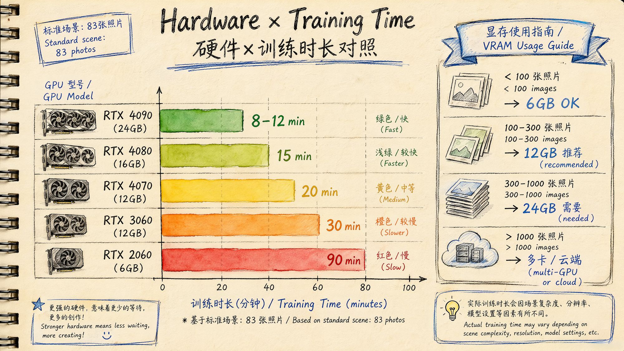
# 1/8 resolutionHardware × Runtime Reference Table
Based on the standard test scene of 83 iPhone 15 photos (4000×3000):
| GPU | VRAM | Training time (30K iter) | Max scene size | Power | Reference price |
|---|---|---|---|---|---|
| RTX 2060 | 6 GB | ~90 min | < 100 images | 160W | ¥1,500 used |
| RTX 3060 | 12 GB | ~30 min | < 300 images | 170W | ¥2,000 |
| RTX 4060 Ti | 16 GB | ~22 min | < 400 images | 160W | ¥3,200 |
| RTX 4070 | 12 GB | ~20 min | < 300 images | 200W | ¥4,000 |
| RTX 4080 | 16 GB | ~15 min | < 500 images | 320W | ¥7,500 |
| RTX 4090 | 24 GB | ~8–12 min | < 1000 images | 450W | ¥13,000 |
| RTX 5090 | 32 GB | ~6–8 min | < 1500 images | 575W | ¥16,000 |
VRAM usage rule of thumb:
VRAM ≈ base overhead (2GB) + image cache (N × resolution × 12B) + Gaussian parameters (M × 200B)• 100 4K images + 1M Gaussians ≈ 6–8 GB
• 300 4K images + 3M Gaussians ≈ 12–16 GB
• 1000 4K images + 5M Gaussians ≈ 20–24 GB
Alternatives if you have no GPU:
| Option | Cost | Speed | Notes |
|---|---|---|---|
| Cloud GPU rental (Vast.ai) | RTX 4090: $0.25/h | Same as local | Hourly billing, best price-performance |
| Google Colab Pro | $10/month | T4/A100 | Time limits and disconnect risk |
| Cloud services (Luma/Polycam) | Free–$8/month | 3–45 min | Easiest, but no parameter tuning |
| OpenSplat CPU mode | Free | ~100× slower | For verification only, not practical |
Training Parameters in Depth
Core Parameter Groups
- Iterations and scheduling
| Parameter | Default | Purpose | Tuning direction |
|---|---|---|---|
| iterations | 30,000 | Total training steps | Bump to 50K for difficult scenes |
| densify_from_iter | 500 | Iteration at which densification begins | Keep default |
| densify_until_iter | 15,000 | Iteration at which densification stops | Lower if you have too many Gaussians |
| densification_interval | 100 | Run densification every N steps | Keep default |
| opacity_reset_interval | 3,000 | Reset opacity every N steps | Keep default |
- Density control (the biggest driver of final quality)
| Parameter | Default | Purpose | Tuning direction |
|---|---|---|---|
| densify_grad_threshold | 0.0002 | Gaussians with gradient above this value get split | Lower → more splits → denser → more VRAM |
| percent_dense | 0.01 | Gaussians larger than 1% of scene scale are split rather than cloned | Keep default |
| min_opacity | 0.005 | Gaussians below this value are pruned | Raise → more aggressive pruning → fewer floaters |
- Learning rates
| Parameter | Initial | Final | Notes |
|---|---|---|---|
| position_lr | 0.00016 | 0.0000016 | Exponential decay, controls how fast Gaussians move |
| feature_lr | 0.0025 | - | Color / SH coefficient learning rate |
| opacity_lr | 0.05 | - | Opacity learning rate |
| scaling_lr | 0.005 | - | Scale learning rate |
| rotation_lr | 0.001 | - | Rotation learning rate |
- Loss function
Total Loss = (1 - λ) × L1_loss + λ × (1 - SSIM)Default λ = 0.2. L1 enforces pixel-level accuracy; SSIM enforces structural similarity.
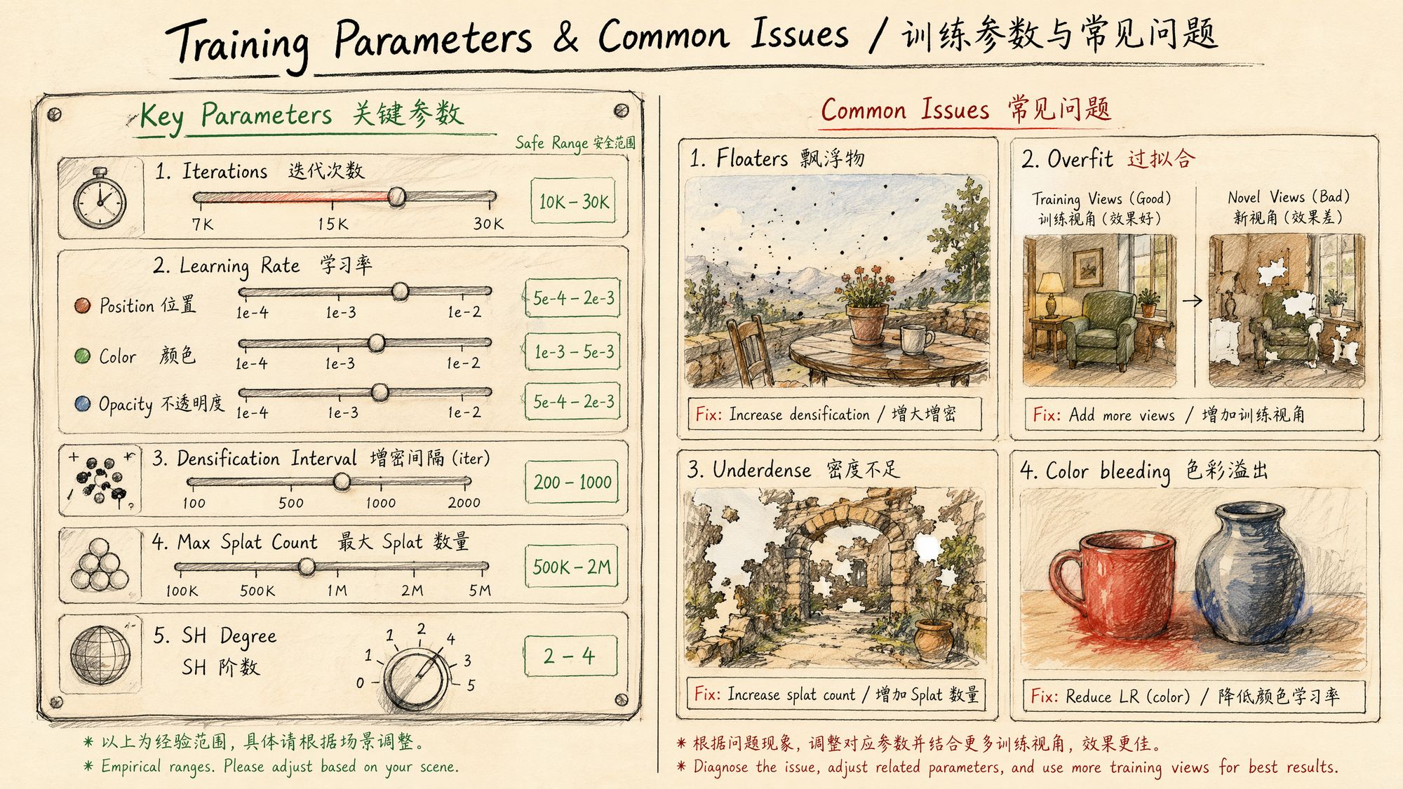
Common Errors and Troubleshooting
Issue 1: Floaters
Symptoms: random colored specks or translucent fog appear in mid-air
Causes:
• Over-densification: gradient threshold too low, Gaussians spawn even in empty regions
• Dust/water droplets/lens smudges in the input images
• Background sky region wrongly reconstructed
Solutions:
# Solution 1: raise the pruning threshold --min_opacity 0.01
# Up from 0.005
# Solution 2: make densification less aggressive --densify_grad_threshold 0.0005
# Up from 0.0002
# Solution 3: use a mask to exclude the sky # Generate a sky mask before training, exclude these regions from the loss
Inside PostShot: after training, use the built-in Crop tool to manually delete floater regions.
Issue 2: Overfitting
Symptoms: looks perfect from training viewpoints, but new viewpoints show severe artifacts
Causes:
• Too few training viewpoints (< 50 images)
• Uneven view coverage (some directions have no images)
• Too many iterations
Solutions:
# Solution 1: reduce iterations --iterations 15000
# Down from 30000
# Solution 2: add regularization # Use Nerfstudio's depth regularization ns-train splatfacto \
--pipeline.model.use-depth-loss True \
--pipeline.model.depth-loss-mult 0.1
# Solution 3: address the root cause—add more training views # Go back to capture and fill in the missing angles
Issue 3: Underdense
Symptoms: visible holes or transparent regions in the scene
Causes:
• Initial point cloud too sparse (COLMAP extracted too few features)
• Densification gradient threshold too high
• Densification stopped too early
Solutions:
# Solution 1: lower the densification threshold --densify_grad_threshold 0.0001
# Down from 0.0002
# Solution 2: extend the densification phase --densify_until_iter 20000
# Up from 15000
# Solution 3: increase initial point-cloud density # Use more feature points in COLMAP colmap feature_extractor --SiftExtraction.max_num_features 16384
Issue 4: Color Bleeding
Symptoms: edge colors of an object bleed into adjacent regions
Causes:
• Gaussians too large, crossing object boundaries
• SH degree too low to model view variation correctly
Solutions:
# Solution 1: cap maximum Gaussian size # Add scale clipping in your training code
# Solution 2: raise SH degree --sh_degree 4
# Up from 3 (increases memory usage)
# Solution 3: use masks to assist training # Generate a mask for foreground objects to keep Gaussians from crossing boundaries
Issue 5: Training Crash / NaN
Symptoms: Loss suddenly becomes NaN or Inf, training stops
Causes:
• Learning rate too high
• Outliers in initial point cloud (very far points)
• Numerical overflow caused by insufficient VRAM
Solutions:
# Solution 1: lower the learning rate --position_lr_init 0.00008
# Halved
# Solution 2: clean the initial point cloud # Remove outliers from the COLMAP output python -c " import pycolmap r = pycolmap.Reconstruction() r.read('./sparse/0/') # Remove points farther than 3 std deviations from center import numpy as np pts = np.array([p.xyz for p in r.points3D.values()]) center = pts.mean(axis=0) dists = np.linalg.norm(pts - center, axis=1) threshold = dists.mean() + 3 * dists.std() # filter... "
# Solution 3: use mixed-precision training # gsplat supports FP16 by default, which can reduce numerical issues
Issue 6: VRAM Insufficient (OOM)
Symptoms: CUDA out of memory error
Solutions in order of priority:
# 1. Lower image resolution (most effective) # Use the images_2/ or images_4/ subdirectory python train.py -s ./data/ --resolution 2
# Use 1/2 resolution
# 2. Limit the number of Gaussians --densify_grad_threshold 0.0005
# Fewer splits # Or set Max Splat Count in PostShot
# 3. Reduce image cache --data_device cpu
# Keep images in CPU memory, load to GPU on demand
# 4. Lower SH degree --sh_degree 2
# Down from 3, saves ~30% memory
# 5. Reduce the number of training images # Uniformly sample 200 from 500
Training Quality Evaluation
Quantitative Metrics
After training, use a test set to evaluate quality:
# Nerfstudio automatic evaluation ns-eval \
--load-config ./output/config.yml \
--output-path ./eval_results.json
# Original 3DGS evaluation python metrics.py -m ./output/my_scene/
Interpretation:
| Metric | Meaning | Excellent | Acceptable | Poor |
|---|---|---|---|---|
| PSNR (dB) | Peak signal-to-noise ratio | > 28 | 25–28 | < 25 |
| SSIM | Structural similarity | > 0.92 | 0.85–0.92 | < 0.85 |
| LPIPS | Perceptual similarity (lower is better) | < 0.10 | 0.10–0.20 | > 0.20 |
Qualitative Checks
Numerical metrics cannot replace human inspection. Below are items you must verify visually:
-
Edge sharpness: are object edges crisp, or are there blurry halos?
-
New-view consistency: from interpolated positions between training views, do you see flicker or popping?
-
Detail preservation: are text and texture details still legible?
-
Floaters: are there colored specks in the air that don't belong to the scene?
-
Transparency: have any regions become transparent that shouldn't be?
Inktoys' Take
On choosing a training tool, here is my hands-on experience:
I have used nearly every tool listed above. My daily workflow has settled on this combination:
Quick preview: Luma AI (shoot on phone, upload directly, see results in 3 minutes, decide whether the scene is worth doing seriously).
Production projects: RealityScan alignment → PostShot training. RealityScan's SfM is 10× faster and more robust than COLMAP, and PostShot's live preview lets me catch problems mid-training and adjust on the fly.
Research / experiments: Nerfstudio splatfacto. When I need to compare methods, test new parameters, or reproduce papers, Nerfstudio's modular design is irreplaceable.
On "how long is enough":
This is the question beginners ask most. The answer is simple: watch the loss curve. When the loss has fallen by less than 1% over the most recent 5,000 iterations, continuing to train is meaningless. For most scenes, that inflection point shows up around 20,000–25,000 iterations.
There is one exception: if your scene has lots of high-frequency detail (foliage, grass, text), it may take 40,000–50,000 iterations to fully converge. At that point SH degree 3 may also be insufficient—try degree 4.
On hardware investment:
If you take 3DGS seriously, the RTX 4090 is currently the best price-performance choice. Its 24 GB of VRAM handles the vast majority of scenes, and it trains 3–4× faster than an RTX 3060. Given the time you save, the investment pays for itself quickly.
If your budget is tight, the RTX 3060 12 GB is the minimum usable configuration. The 6 GB RTX 2060 can technically run training, but you will spend a great deal of time downscaling resolution, capping Gaussian counts, and fighting OOM—time you could have spent on more valuable work.
In one sentence: training is the most "automated" stage of the 3DGS pipeline—once the upstream prep is done right, training itself is just clicking start and waiting. Spend your energy on capture and SfM; 90% of the problems that surface during training are upstream errors becoming visible.
Further Reading
• Kerbl, B. et al. (2023). "3D Gaussian Splatting for Real-Time Radiance Field Rendering." SIGGRAPH.
• Ye, V. et al. (2025). "gsplat: An Open-Source Library for Gaussian Splatting." JMLR.
• Kheradmand, A. et al. (2024). "3D Gaussian Splatting as Markov Chain Monte Carlo." NeurIPS.
• Bulo, S. R. et al. (2024). "Revising Densification in Gaussian Splatting." CVPR.
• PostShot official documentation: https://jawset.com/postshot/docs
• Nerfstudio splatfacto documentation: https://docs.nerf.studio/
• LichtFeld Studio GitHub: https://github.com/MrNeRF/LichtFeld-Studio
• gsplat documentation: https://docs.gsplat.studio/